This is Part 6 of the Spark SQL Metrics deep-dive series:
- Part 1: Metric types, complete reference, and what they mean
- Part 2: How metrics work internally, and how AQE uses them for runtime decisions
- Part 3: Extension APIs, UI rendering, and REST API
- Part 4: How Gluten extends the metrics system
- Part 5: Gluten metrics internals — node mapping, pipeline aggregation, MetricsUpdaterTree
- Part 6 (this post): Metrics in action — a real-world TPC-DS q99 walkthrough with Gluten/Velox
In Parts 1–5, we built up all the machinery: metric types, internal plumbing, extension APIs, Gluten’s architecture, and native-side aggregation. Now it’s time to put it all to use. We’ll open the Spark UI for a real query, walk through every operator’s metrics, and show exactly how to read them to understand what happened during execution.
The Query: TPC-DS q99
TPC-DS q99 is a 5-table join query that analyzes catalog sales shipping delays by warehouse, ship mode, and call center. It groups shipments into buckets based on how late they arrived (31–60 days, 61–90 days, 91–120 days, and over 120 days), then ranks the results.
We ran this query at scale factor 10,000 (10 TB of raw data) on a cluster using Gluten/Velox as the native execution backend, with Delta Lake tables on cloud object storage.
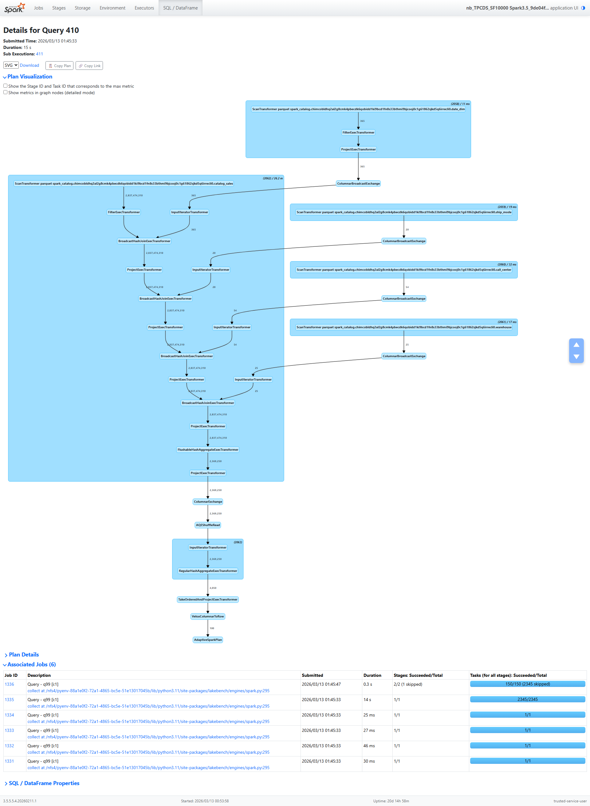
The query plan follows a classic star-schema pattern:
catalog_sales (fact table, 3.3B rows)
  → BroadcastHashJoin with date_dim
  → BroadcastHashJoin with ship_mode
  → BroadcastHashJoin with call_center
  → BroadcastHashJoin with warehouse
  → Partial HashAggregate
  → Shuffle (hash partitioning)
  → AQE Coalesce
  → Final HashAggregate
  → TakeOrderedAndProject (top 100)
Every number in this post is real. Let’s walk through the metrics, operator by operator, and see what they tell us.
Section 1: The Fact Table Scan — 3.3 Billion Rows
The first operator in the plan is ScanTransformer catalog_sales. This is where everything starts, and the metrics here tell a rich story.
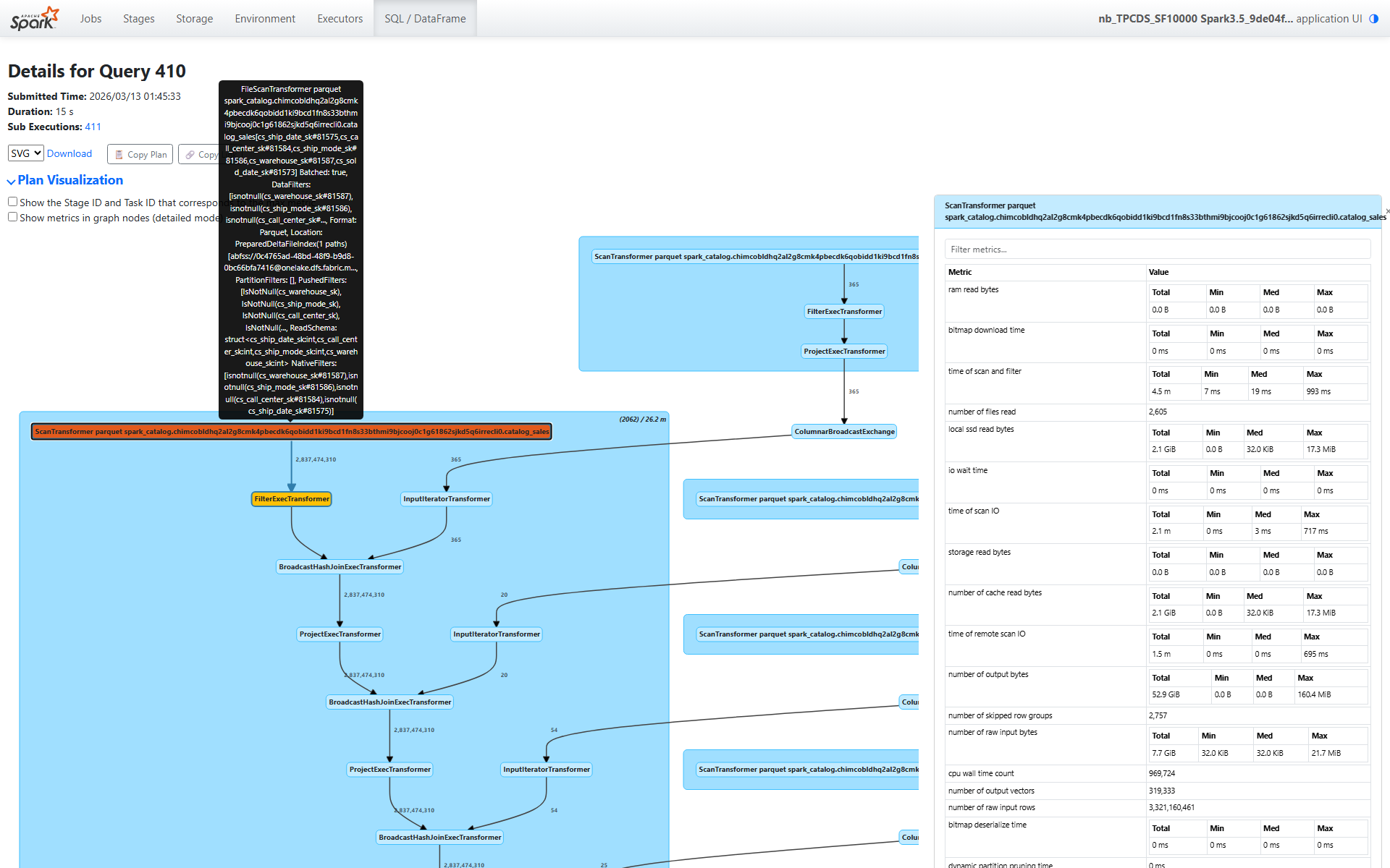
Scale
number of raw input rows: 3,321,160,461 — 3.3 billion rows in the catalog_sales tablenumber of output rows: 2,837,474,310 — 2.8 billion rows after predicate pushdown eliminates non-matching row groupssize of files read: 910.9 GiB across 2,605 files spanning 1,837 partitions
That’s a massive scan. But look at how efficiently it was served.
The I/O Tier — A Cache Story
This is where it gets interesting:
storage read bytes: 0.0 B — zero bytes from remote storagelocal ssd read bytes: 2.1 GiB — all data served from local SSD cacheram read bytes: 0.0 B — no in-memory cache hitsnumber of cache read bytes: 2.1 GiB — matches the local SSD number exactly
Think about what this means: the table occupies 910.9 GiB on disk, but we only needed to read 2.1 GiB of actual data. That’s a 99.8% reduction. Two things made this possible:
- Columnar format efficiency — we only read the columns referenced by the query (a fraction of the table’s total columns)
- Predicate pushdown to row groups — Parquet/Delta statistics let Velox skip entire row groups whose min/max ranges don’t match the filter predicates
And all 2.1 GiB came from local SSD cache — not a single byte traversed the network to remote storage.
Row Group Pruning
number of skipped row groups: 2,757
Velox examined row group statistics and skipped 2,757 row groups entirely. These row groups contained data outside the predicate ranges (the date_dim filter constrains d_month_seq to a specific range, which translates to a range on cs_sold_date_sk). This is the primary reason we read only 2.1 GiB from 910.9 GiB of files.
Dynamic Filters
number of dynamic filters accepted: 9,380
This is a powerful optimization. During execution, the build side of each broadcast hash join produces a filter (a set of join key values or a Bloom filter). These filters are pushed back down to the scan operator at runtime. With 9,380 dynamic filters applied, the scan eliminated rows that would never match any join — before the rows even reached the join operators.
If you’ve read Part 4, you know Gluten instruments dynamic filter acceptance at the scan level. This metric tells you: yes, runtime filters were generated and applied, and they helped.
Timing
time of scan and filter: 4.5 minutes total across all taskstime of scan IO: 2.1 minutes — about half the scan time was I/O waitcpu wall time count: 969,724 batches processed
The scan processed nearly a million batches. The I/O time (2.1 min) versus total scan time (4.5 min) tells us that roughly half the time was I/O and half was CPU work (decompression, predicate evaluation, column extraction).
Task Distribution
Looking at the min/median/max breakdown:
- Bytes read per task: median 32 KiB, max 17.3 MiB — moderate skew in data distribution
- Peak memory per task: median 32 KiB, max 29.9 MiB
Most tasks process small amounts of data (the table is split across 1,837 partitions), but some partitions are significantly larger. This is typical for real-world data — perfectly uniform partitioning is rare.
Section 2: The Four Broadcast Hash Joins — 2.8 Billion Probe Rows
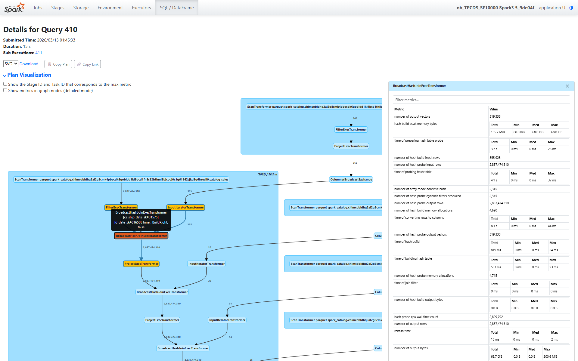
After the scan, the plan chains four broadcast hash joins. Each joins the fact table with a dimension table: date_dim, ship_mode, call_center, and warehouse. Let’s walk through the date_dim join (node [18]) in detail, then summarize the pattern across all four.
Build Side (date_dim)
number of hash build input rows: 855,925 (date_dim rows replicated across partitions via broadcast)time of hash build: 819 ms total — fast, small dimension tabletime of building hash table: 533 ms — actual hash table constructionhash build peak memory bytes: 155.7 MiB total (68 KiB per task — tiny)
The build side is trivially small. date_dim has a few hundred thousand rows, and after broadcast, each task gets a copy. Building the hash table takes well under a second.
Probe Side
Now the probe side — this is where the work happens:
number of hash probe input rows: 2,837,474,310 — the entire 2.8 billion row output from the scantime of hash probe: 31.4 seconds totaltime of probing hash table: 4.1 seconds — actual hash lookupstime of preparing hash table probe: 3.7 seconds — deserializing the broadcast datatime of converting rows to columns: 8.3 seconds — columnar format conversion
Notice the breakdown: out of 31.4 seconds of total probe time, only 4.1 seconds was spent on actual hash lookups. The rest was overhead — deserialization, format conversion, and pipeline coordination. This is typical for broadcast joins: the hash lookup itself is fast (the hash table fits in L2/L3 cache), but marshaling 2.8 billion rows through the pipeline takes time.
Dynamic Filters Generated
number of hash probe dynamic filters produced: 2,345
Each task that processes this join produces a dynamic filter from the build side’s key values. These 2,345 filters are pushed back to the scan operator (contributing to the 9,380 dynamic filters we saw earlier — multiple joins contribute filters).
No Spill
bytes written for spilling of hash build: 0.0 Bbytes written for spilling of hash probe: 0.0 B
Perfect. The dimension tables are small enough to fit entirely in memory. No data was spilled to disk during any join.
Output
number of hash probe output rows: 2,837,474,310 — all 2.8 billion rows pass through- Output data volume: 65.7 GiB (the output grows because we’ve added columns from the dimension table)
All rows pass because the predicate pushdown and dynamic filters already eliminated non-matching rows during the scan. The join itself is just enriching each row with dimension attributes.
Pattern Across All Four Joins
Here’s a summary of all four broadcast hash joins side by side:
| Join | Build Table | Build Rows | Probe Time | Post-Projection Time |
|---|---|---|---|---|
| date_dim | date_dim | 855,925 | 31.4s | 8.1s |
| ship_mode | ship_mode | 46,900 | 1.6 min | 8.0s |
| call_center | call_center | 126,630 | 2.4 min | 8.1s |
| warehouse | warehouse | 58,625 | 2.8 min | 8.2s |
Notice how the probe time increases with each successive join. This isn’t because later joins are slower — it’s because wallNanos (which backs the probe time metric) includes child operator wait time. As we explained in Part 4, each operator’s wall time includes the time spent waiting for data from its child operators. The warehouse join (the outermost) includes the time of all three joins below it, plus the scan.
The post-projection time is remarkably consistent (~8 seconds each), which makes sense — each join appends a few columns, and the projection work is proportional to output size, which is roughly the same (2.8B rows) at each stage.
Section 3: The Aggregation — 2.8B → 2.3M Rows
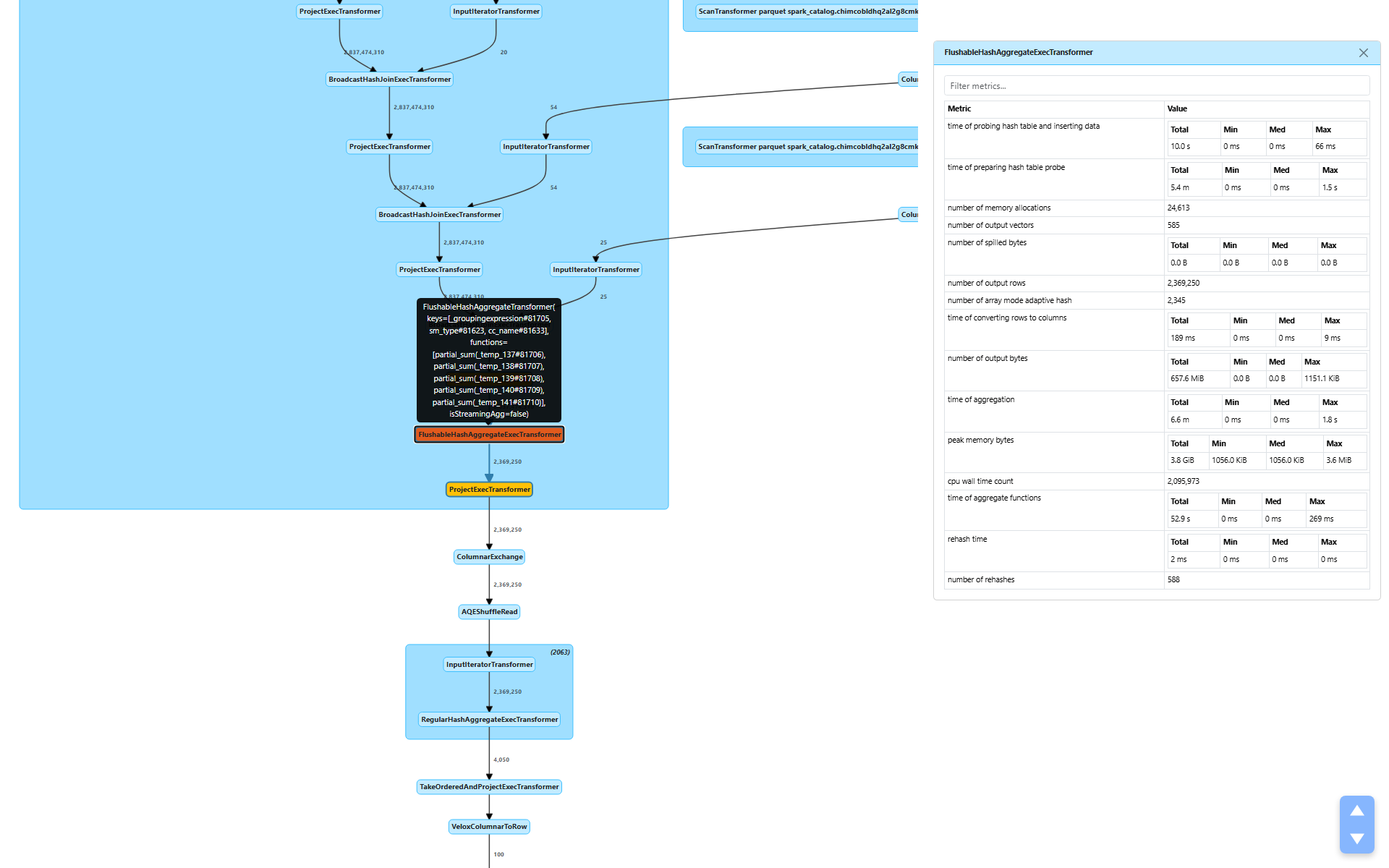
After the four joins, the plan applies a FlushableHashAggregateExecTransformer (node [10]) for partial aggregation. This is where the data volume drops dramatically.
number of output rows: 2,369,250 — a 1,200× reduction from 2.8 billion input rowstime of aggregation: 6.6 minutestime of aggregate functions: 52.9 seconds — the actual SUM() computationstime of preparing hash table probe: 5.4 minutes — dominated by child operator wait time (the joins above)peak memory bytes: 3.8 GiB total (max 3.6 MiB per task)number of spilled bytes: 0.0 B — no spill needednumber of output vectors: 585 — only 585 output batches from 2.8 billion input rows
The 1,200× reduction tells us that the group-by keys (warehouse, ship_mode, call_center, date bucket) have high cardinality but still produce far fewer groups than input rows. The actual aggregate computation (SUM) took only 52.9 seconds — the bulk of the 6.6-minute aggregation time is child wait time cascading up from the scan and joins below.
WholeStageCodegenTransformer
The entire native pipeline — from scan through all four joins through partial aggregation — runs inside a single WholeStageCodegenTransformer:
duration: 26.2 minutes total (max 6.6 seconds per task)
This is the end-to-end time for the native execution pipeline. It encompasses everything we’ve discussed so far: scanning 3.3 billion rows, four broadcast hash joins on 2.8 billion rows, and partial aggregation down to 2.3 million rows — all executed in Velox’s vectorized native engine.
Section 4: The Shuffle — Hash-Based, Compact
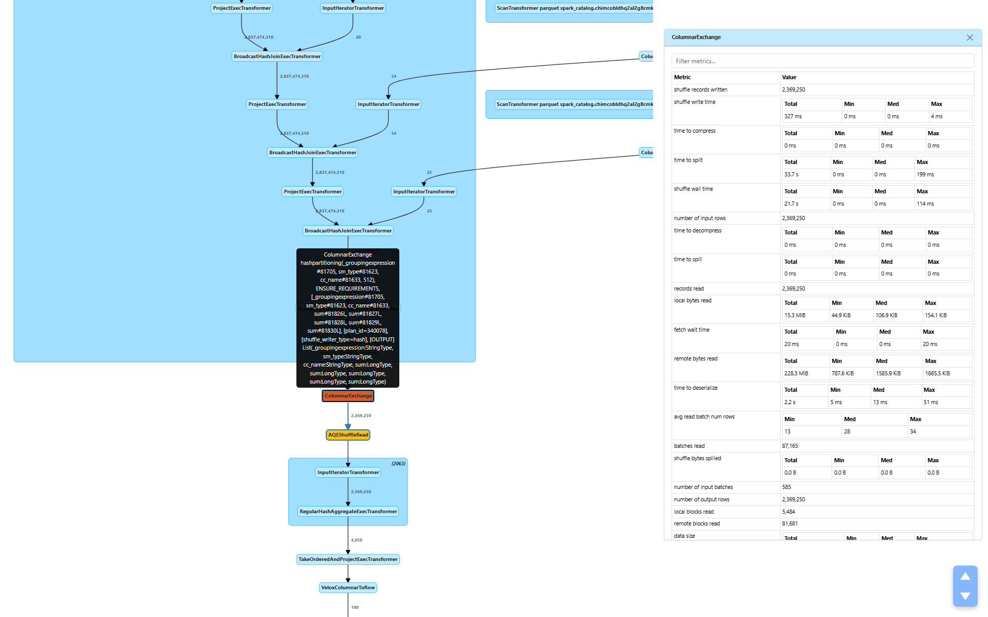
After partial aggregation, the plan shuffles data via ColumnarExchange (node [7]) to redistribute rows by their group-by keys for final aggregation.
Write Side
shuffle bytes written: 243.6 MiB — remarkably smallshuffle write time: 327 mstime to split: 33.7 seconds — hash partitioning into 512 partitionsshuffle wall time: 21.7 secondsshuffle bytes spilled: 0.0 B — everything fits in memorypeak bytes allocated: 255.1 GiB total (446.5 MiB max per task)
The aggregation reduced 2.8 billion rows to 2.3 million rows, and those 2.3 million rows serialize to just 243.6 MiB. Compare that to the 910.9 GiB fact table we started with — the aggregation made the shuffle almost trivially small.
The split time (33.7s) is the time to hash-partition the output into 512 buckets. The actual write time (327 ms) is fast because there’s so little data to write.
Read Side
remote bytes read: 228.3 MiBlocal bytes read: 15.3 MiBremote reqs duration: 41.9 seconds — cross-node shuffle fetchtime to deserialize: 2.2 seconds
Most of the shuffle data (228.3 MiB) was read from remote executors, with a small fraction (15.3 MiB) from local tasks. The 41.9 seconds of remote request duration includes network latency and scheduling overhead — this is typical for cross-node shuffle on a distributed cluster.
The shuffle writer type is hash (visible in the plan), meaning rows are hash-partitioned by the group-by keys for the final aggregation.
Section 5: AQE in Action — 512 → 149 Partitions
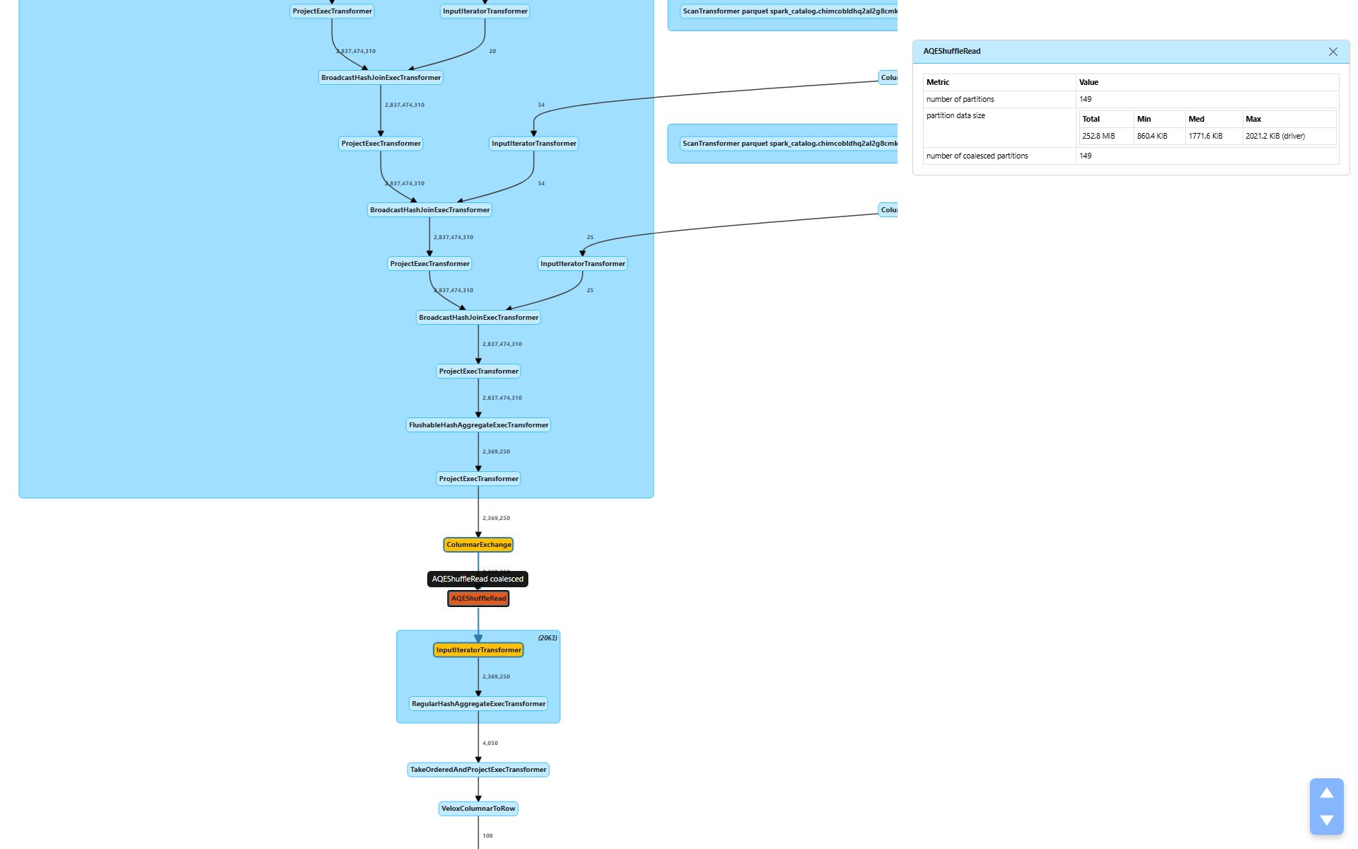
After the shuffle, AQEShuffleRead (node [6]) kicks in:
number of coalesced partitions: 149 — AQE merged 512 partitions down to 149partition data size: 252.8 MiB total, target ~1.7 MiB per partition
AQE examined the shuffle output statistics and determined that 512 partitions was too many for 252.8 MiB of data. At 512 partitions, each partition would average under 500 KiB — not worth the scheduling overhead of 512 tasks. By coalescing to 149 partitions, each task processes a more reasonable ~1.7 MiB.
No skewed partitions were detected (numSkewedPartitions is absent), so AQE only applied coalescing, not skew handling.
This is a perfect example of Part 2’s discussion of how AQE uses metrics for runtime decisions. The shuffle write statistics from Stage 1 directly informed Stage 2’s partition count.
Section 6: Final Aggregation and Result — 4,050 → 100 Rows
Final Aggregation
RegularHashAggregateExecTransformer (node [4]) performs the final merge of partial aggregates:
- Input: 2,369,250 rows across 149 tasks
number of output rows: 4,050 — the final group counttime of aggregation: 3.2 secondspeak memory bytes: 194.4 MiB (1.3 MiB per task)- No spill
The partial aggregation already did the heavy lifting — the final aggregation just merges pre-aggregated groups. 2.3 million partial rows collapse to 4,050 final groups in 3.2 seconds. Trivial.
Top-100 Sort and Result Delivery
TakeOrderedAndProjectExecTransformer takes the 4,050 rows, sorts them, and returns the top 100. Then VeloxColumnarToRow converts the columnar result to row format for the driver:
number of output rows: 100
From 3.3 billion rows to 100. That’s the entire query.
The Full Picture — What the Metrics Tell Us
Let’s step back and see the complete execution flow with key metrics:
Scan catalog_sales: 3.3B raw → 2.8B rows (4.5 min, 2.1 GiB from SSD cache)
  ↓ 9,380 dynamic filters applied, 2,757 row groups skipped
Join × 4 (broadcast): 2.8B rows through each join, zero spill
  ↓
Partial Aggregation: 2.8B → 2.3M rows (1,200× reduction)
  ↓ WholeStageCodegenTransformer: 26.2 min total native pipeline time
Shuffle: 243.6 MiB written (hash, 512 partitions)
  ↓
AQE: 512 → 149 partitions (coalesced)
  ↓
Final Aggregation: 2.3M → 4,050 rows (3.2s)
  ↓
Top-100 Sort → 100 rows returned
Key Takeaways from the Metrics
1. Cache is king. Zero bytes from remote storage, everything from local SSD. The 910.9 GiB table only needed 2.1 GiB of actual reads — a 99.8% reduction through columnar format efficiency and predicate pushdown.
2. Row group pruning is effective. 2,757 row groups skipped. Velox used Parquet/Delta min-max statistics to eliminate entire row groups before reading a single byte from them. This is the primary driver of the I/O reduction.
3. Dynamic filters work. 9,380 filters applied during the scan, generated at runtime from join build sides. These filters eliminated rows before they even reached the join operators, avoiding unnecessary processing of billions of rows.
4. No spill anywhere. Joins, aggregations, and shuffle all fit in memory. Zero bytes spilled to disk across the entire query. The dimension tables were small enough for broadcast, and the partial aggregation reduced data volume before the shuffle.
5. AQE coalescing helps. 512 → 149 partitions for the final aggregation. Without AQE, we’d have 512 tasks each processing less than 500 KiB — wasteful scheduling overhead for a trivial amount of data.
6. The bottleneck is the native pipeline. 26.2 minutes in WholeStageCodegenTransformer, encompassing the scan of 3.3 billion rows, four joins on 2.8 billion rows, and partial aggregation. This is where the real work happens, and it’s all executed in Velox’s vectorized native engine.
7. wallNanos increases up the tree. Each parent operator’s wall time includes its children’s wait time. The outermost join shows 2.8 minutes not because it’s slow, but because it includes the scan, three inner joins, and all their I/O. This confirms the caveat from Part 4 — always read wall time metrics with the operator tree in mind.
Wrapping Up
This walkthrough demonstrates that metrics aren’t just numbers on a screen — they’re a narrative. Every metric answers a specific question:
- Where did the data come from? → I/O tier metrics (all from SSD cache)
- How much work was avoided? → Row group pruning and dynamic filters
- Where did the data volume drop? → Aggregation (1,200× reduction)
- Was there any resource pressure? → Spill metrics (zero everywhere)
- Did the optimizer help? → AQE coalescing (512 → 149 partitions)
When you next open the Spark UI for a slow query, you now have the vocabulary to read every metric, understand what it means, and pinpoint exactly where the bottleneck is.
In Part 1, we learned the five metric types and built a complete reference. In Part 2, we traced how metrics flow through the Spark internals and how AQE uses them. In Part 3, we explored the extension APIs, UI rendering, and REST endpoints. In Part 4, we saw how Gluten extends the metrics system for native execution. In Part 5, we went deep into Gluten’s native-side metrics machinery. And in Part 6 (this post), we put it all together — walking through a real TPC-DS query to show how every metric tells part of the execution story. This concludes the series.